Return to main Astrophotos page
Motivation
I've been involved in amateur astronomy since the eighth grade, when my science teacher got me excited about the hobby. I started with my parents' binoculars, moved up to a refractor, and soon got a larger reflector. I enjoyed visual observing for a number of years, but found eventually that I was looking at the same (relatively bright) objects over and over again. For the numerous fainter objects in the catalogs, the most I could say was that I managed to detect them, usually with averted vision. I wanted to try astrophotography for a long time, but it was a number of years before I obtained a tracking mount and a telescope that is compatible with the focal requirements of prime-focus photography. Since I obtained this equipment, I have found astrophotography to be quite satisfying for several reasons. First, it provides a way to really "see" the fainter details of objects. Second, it generates raw data that I can process in a way that shows the object as close to its actual appearance as possible. Finally, it creates a kind of souvenir of many of the objects I have seen visually.
Outings
When I was in high school in Arizona, I went with my dad to a number of star parties near Arizona City that were organized by the East Valley Astronomy Club. Since I moved to California, initially for graduate school, I have gone many times to Calstar at Lake San Antonio (my favorite site for astrophotography), a few times to the Golden State Star Party (dark but windy - bad for my photography setup), a number of times to Monte Bello (nearby but not very dark), to Houge Park in San Jose for SJAA events, and a few other places out of town. Sometimes I just set up in Palo Alto, but the sky here is quite bright, so it's not good for much beyond planets, the ring nebula, or globular clusters. I went on almost all of these outings with my wife Kathy, who not only makes the trips a lot more fun, but helps in many ways including packing the equipment, setting up camp, suggesting interesting objects from the catalog, and helping to run the equipment.
Telescopes
Most of the photos on this page were taken with an 8″, f/6 Newtonian. The primary mirror orginated from a kit (Newport Glass), and I started working on it in the fall of 2002 when I had 6 weeks off. I got through the grinding and started polishing, but eventually realized that there were still some pits left over that should have been removed in the finer grinding stages. I started working on this again in 2005, in the SJAA mirror-making class run by Mike Koop. I went back and redid the fine grinding, and started the polishing all over again. Eventually (2006) I finished figuring the mirror. According to the Focault test, the figure is better than lambda/10. However, I am skeptical of this result because I can see some difference in the ring patterns for star images inside and outside of focus. The rest of the telescope includes a cardboard tube, a University Optics mirror cell, an Antares secondary mounted with curved supports (that is why there are no clear rays in the star images), a 2″ focuser, a Telrad, and a cradle that holds the telescope and allows it to be rotated about the optical axis. Thanks to Tom Frederickson for designing and making the essential parts for this cradle, and for help with the rest of the assembly.
A few of the photos were taken with an 8″, f/9 Newtonian on a Dobsonian mount that I've had since high school. This is a home-made telescope that we found through a newspaper ad. It has a Cave mirror, but in its original condition had some problems including astigmatism. We took it to Pierre Schwaar (around 1991) who diagnosed the mirror problem (it was due to mounting stress from excessive glue), remounted it, and also redid the secondary mount. Since then this telescope has worked quite well for observing planets.
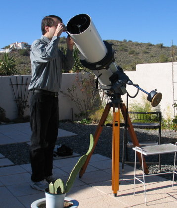
Most recently, I started using a C14 (14″ Schmidt-Cassegrain) telescope. Usually I combined this with a focal reducer lens that takes the focal ratio from f/11 down to f/7. This telescope gathers 3 times more light, and can possibly give higher resolution under good seeing conditions, but it also increases the tracking challenges. Due to the reduced field of view with a given camera, it is best suited for more compact objects.
Mounts
5/2008 - 4/2010: Meade LXD55 equatorial mount bought at an SJAA swap meet. This mount was in rough shape initially, and it took a lot of work to get it into working condition. It had a WarpsDrive belt kit installed, but the pulleys did not line up and they were scraping against the plastic case, and there was no easy fix because there wasn't enough room inside the case for the pulleys. Eventually I got it functioning through a combination of countersinking a screw hole on the gear box and removing some plastic from the case. For photography, the tracking was such that I could take 10s exposures (open-loop) and get mostly good images. For 30s exposures, maybe half of the images were good, and for 60s exposures only about 1/4 of the images were good.
5/2010 - : Orion Atlas EQ-G equatorial mount, bought at SJAA auction. This is a much heavier mount, and it drives quite a bit better, with less backlash. The open-loop tracking is marginally better than with the LXD55 mount, but without guiding I'm still limited to 20-60s exposures.
10/2021 - : Losamndy G11T equatorial mount. This mount is much heavier still, but I got it to handle the new C14 telescope.
Cameras
Starshoot DSCI: Orion Starshoot Deep Space Imaging Camera bought used off of Astromart. This camera has some problems but was cheap. It uses a Sony ICX259AK CCD chip with cyan, yellow, green and magenta pixels arranged in a 2x4 tile. The individual pixels are 6.50 x 6.25 microns, corresponding to 1.117 X 1.074 arcseconds per pixel at prime focus of the 8″, f/6 scope. The camera has a TE cooler which gives some improvement to the dark current, but we did not use it at Calstar because it is a power hog, and I did not want to risk depleting our limited battery supply, which was also needed to power the mount. Except for the TE cooler, the camera is powered entirely through the USB cable.
ST-4000XCM: In pursuit of better imaging of fainter fuzzies, I more recently obtained this camera from SBIG. It is also a single-shot color camera, but its main advantages over the Starshoot are (1) a much larger sensor, (2) software control over the TE cooler, and (3) a second CCD sensor that can be used for guiding. The first deep-sky image I obtained with it (and first ever image with guiding!) was of M81. The camera uses the Kodak KAI-4022CM CCD chip, which has 2048x2048 subpixels, 7.4 microns square, corresponding to 1.272 arcseconds per pixel at 1200mm focal length. The subpixel filters follow a blue, green; green, red arrangement in a 2x2 tile.
Philips SPC 900NC Webcam: I bought this camera at a swap meet to image planets. It provides higher frame rates and smaller pixel sizes but also has some fairly noticeable imaging defects.
Allied Vision Alvium 1800 U-319m: This is a monochrome CMOS camera with a global shutter, low readout noise, and a fairly small 3.45μm pixel size. I have recently started experimenting with this camera on stars, planets, and other small, bright objects where I want to maximize resolution.
Image Processing
Most of the final images shown here were created by combining many shorter exposures ("stacking") to improve the signal-to-noise ratio. For the unguided images (using the Starshoot camera) the exposure times were typically in the range of 10-30 seconds. For the more recent guided images (ST-4000XCM) the exposures are longer, usually 5 minutes each. I did most of the image processing in an automated way using code that I wrote originally in Matlab. In 2013, I converted this to stand-alone applications written in C, using functions from the OpenCV image processing library where possible. The steps in the current procedure are (1) identify bad pixels (the ~0.1% of pixels with the highest dark current) from the dark frames. (2) For each raw image, subtract a background (using the dark frames). (3) Divide by a flat field image, if available. (4) Convert to a grayscale image by 2x2 binning (5) Compare the grayscale image with the grayscale image from the first exposure in the set to determine a relative shift and rotation. This is done by finding the maximum of the cross-correlation function. Changes in image rotation usually result from mechanical problems (the camera moving in the eyepiece holder, or the tube rolling in its cradle) but could also result from poor polar alignment. (6) Returning to the raw color image, determine separate shifts for the different color subpixels, again using the cross-correlation method. These corrections are necessary because of atmospheric refraction, and are especially important for objects low in the sky. (7) Find cosmic rays and mark them as bad pixels. (8) Remove streaks due to satellites as specified manually in the configuration file. (9) Applying the shifts and rotations, add each of the color channels to a total for each channel, keeping track of the total time contributions made for each pixel, omitting the bad pixels. (10) In the final totals, check for pixels that received insufficient contributions in one or more color channel, and fill them in using neighboring pixels. For the unguided sets containing a large number of frames, this was only necessary for pixels near the edges. But for guided sets containing just a few exposures this interpolation is usually done across the whole image. (11) On a pixel-by-pixel basis, divide the total intensity by the total exposure time. (12) Remove an additional background for each color channel, typically estimated as a threshold such that 10% of the pixels are below this threshold. The background can be spatially constant (1 fit parameter), linear (3 fit paramters), or quadratic (6 fit parameters), depending on the availabilty of known dark locations that can be used for fitting. (13) Convert the color channel data to RGB using a color calibration matrix. For each camera, the same matrix was used for all objects, and this matrix has been tested with a color test pattern and appears to give fairly true color results. (14) At this point the image exists as a floating-point array, which needs to be converted to an integer format for display. The original image can have a very large dynamic range, such that it is impossible to display all of the object's features on a normal computer display. Nevertheless, I generally chose to use a linear scaling, since this retains a true sense of the large intensity contrast present in the object. To show the whole dynamic range, I normalize the intensity to several different levels for each object, generating separate images. The original image is divided by the parameter "Imax" shown underneath each thumbnail below, and any intensities below 0 or above 1 are clipped. By displaying several images in this way, it is possible to see, for example, that M31 has a very small and bright central core. In older photographs, this part of the galaxy is usually saturated so that this central structure cannot be seen at all. In recent images, the galaxy is usually scaled nonlinearly, so the central structure can be seen, but you would have no way to know that it is hundreds of times brighter than the outer spiral arms. More recently, I have started including some nonlinearly scaled images as well, using either a histogram equalization-type method or a logarithmic scaling. Such images are labeled 'nonlinear' and cannot be compared quantitatively to the other images.
As of fall, 2014, I have started using flat field images to correct for variations in the combined telescope/sensor efficiency across the image. In the first experiments, I tried either shining a light at a sheet of paper held in front of the telescope, or taking images of the blue sky before it gets completely dark. The second method (blue sky) worked much better. The only disadvantage of this method is that, if I recollimate the telescope later in the night (based on the coma radiating from an off-center point), there might still be uncorrected nonuniformity. In processing the flat field data, the different color subpixels are combined, so that the flat field correction does not affect the color. Flat field correction is especially important when imaging fainter objects requiring many hours of exposure. Since the sky glow can be much brighter than the target object, incorrectly subtracting the sky glow background can lead to major flaws in the image.Other comments
Each image in a set of thumbnails shown side-by-side is obtained from the same data. The parameter Imax corresponds to the intensity, measured in counts per second, that will saturate an image, as explained above. For a given camera, the same image processing procedure was used on all of the data sets, so the colors and intensities (for the same Imax parameter) for different objects can be compared directly, regardless of the number or duration of exposures. The only exception is for the images labeled "3X" - in this case a 3X Barlow lens was used, so the intensity per pixel should be reduced by a factor of 9. Also, there are a few images obtained by other means (for example Mars and Venus), and these do not have an Imax value.
My goal here was to present the images as data (what the object would actually look like), rather than as art, and all of the processing steps described above are designed to remove known artifacts of the imaging system. These steps are fairly standard and are done to remove known camera defects, to subtract skyglow, and hopefully produce the truest possible image. However, since the camera is different from your eye (for example it has better sensitivity to hydrogen alpha emission in the deep red part of the spectrum) some objects, especially emission nebulae, may appear different from what your eye could ever see. Also, because of the stacking procedure described above, the edges of the images typically receive much less signal contribution and therefore appear more noisy. However, I chose not to crop some of the images because the edges contain useful information (bright stars, for example).